6. Decision models¶

Approve, deny, or ask a person. Paying a refund the rules forbid costs the price of the item; refusing one the rules allow costs a customer; a person's review costs a few dollars of their time. By the end you will have a decision model that reads the facts, applies the rules exactly, knows when it isn't sure, and chooses the action with the lowest expected cost, all measured in dollars.

Can you skip this one? If you can answer these, jump to tutorial 7. The answers are at the bottom.

A model is right 97% of the time. Why might it still be the wrong one to let decide?
Five votes say "approve" four times. For a $400 espresso machine, do you approve? For a $12 mug?
What do you gain by letting the model read the facts and R apply the rules, instead of letting the model decide?
Five votes all agree. Why isn't that the same as a probability of 1, and what kind of model gives you a real one?

What you need¶

This tutorial uses rpart (it comes with R) and rpart.plot, parsnip and rsample (install.packages(c("rpart.plot", "parsnip", "rsample"))). One section uses TypeSafe's Jev, which needs a TYPESAFE_API_KEY from console.typesafe.ai in your ~/.Renviron. It costs about seven cents.

library(functai)
library(dplyr)
library(ggplot2)

log_folder <- tempfile("functai-calls-")
ai_config(lm = "gpt-6-luna", log_calls = log_folder)

A decision is a choice with costs¶

The refund desk of tutorials 4 and 5 again: 120 requests, each with the decision the shop's rules give (?refunds).

refunds |> select(item, price, days_since_delivery, final_sale, state, decision)

# A tibble: 120 × 6
   item                 price days_since_delivery final_sale state      decision
   <chr>                <dbl>               <int> <lgl>      <fct>      <fct>   
 1 wall clock           28.5                   66 FALSE      wrong_item deny    
 2 floor rug            39.2                   28 FALSE      wrong_item approve 
 3 stand mixer           9.38                   9 FALSE      faulty     approve 
 4 ceramic planter     139.                    57 FALSE      faulty     approve 
 5 bath towels          75.9                  368 FALSE      used       deny    
 6 desk chair          389.                    17 FALSE      faulty     approve 
 7 cast-iron casserole 458.                    26 FALSE      opened_un… approve 
 8 teapot               11.6                   28 TRUE       wrong_item approve 
 9 pillow pair         129.                    25 FALSE      faulty     approve 
10 ceramic planter      50.0                   94 FALSE      unopened   deny    
# ℹ 110 more rows

Accuracy treats every mistake the same. The desk doesn't. There are two ways to be wrong and one way to be careful:

approving a refund the rules forbid: the shop loses the price of the item;
denying a refund the rules allow: the customer complains, disputes the charge and doesn't come back. Call it $40;
sending it to a person, who reads it and gets it right: five minutes of their time, about $4.

Those numbers are the shop's to set, and they are the most important part of the model. Write them down as code:

review_cost <- 4       # a person reads it
lost_customer <- 40    # a wrong "no"

cost_of <- function(action, decision, price) {
  case_when(
    action == "review"  ~ review_cost,
    action == decision  ~ 0,
    action == "approve" ~ price,          # paid what the rules don't allow
    action == "deny"    ~ lost_customer)  # refused what they do
}

outcome <- function(action, strategy) {
  action <- as.character(action)
  tibble(strategy = strategy,
         reviews = sum(action == "review"),
         wrong_approvals = sum(action == "approve" & refunds$decision == "deny"),
         wrong_denials = sum(action == "deny" & refunds$decision == "approve"),
         dollars = sum(cost_of(action, refunds$decision, refunds$price)))
}

Before any model, three strategies anyone could follow:

n <- nrow(refunds)
baselines <- bind_rows(
  outcome(rep("approve", n), "approve everything"),
  outcome(rep("deny", n), "deny everything"),
  outcome(rep("review", n), "a person reads everything")
)
baselines

# A tibble: 3 × 5
  strategy                  reviews wrong_approvals wrong_denials dollars
  <chr>                       <int>           <int>         <int>   <dbl>
1 approve everything              0              58             0   7114.
2 deny everything                 0               0            62   2480 
3 a person reads everything     120               0             0    480

A person reading everything is the benchmark to beat: never wrong, and $480 for 120 requests. A model has to be cheaper than that including the cost of its mistakes.

The model decides¶

Tutorial 4's function, with the rules in its description:

refund_rules <- ai(decision ~ message + price + days_since_delivery + final_sale,
  "Should the shop refund this request? Follow the refund rules exactly:
  - Damaged on arrival, or the wrong item (or part of the order missing): refund within 60 days
    of delivery, final sale or not.
  - Faulty (it failed in normal use): refund within 365 days, final sale or not.
  - Unopened, or opened but not used, and no longer wanted: refund within 30 days, never for a
    final-sale item.
  - Used and no longer wanted: no refund.",
  .data = refunds, .name = "refund")

direct <- with(refunds, refund_rules(message, price, days_since_delivery, final_sale))
outcome(direct, "the model decides")

# A tibble: 1 × 5
  strategy          reviews wrong_approvals wrong_denials dollars
  <chr>               <int>           <int>         <int>   <dbl>
1 the model decides       0               1             0    13.3

Compare that with the person reading everything. And ask the question a manager would ask about each decision: why? The function answered "approve" or "deny". It can't show its work in a form you could audit, and if the policy changes next month, you'd change a paragraph of prose and hope.

The model reads, R decides¶

Split the job in two. The part that needs reading (what state is the item in?) goes to the model, which is good at it: tutorial 5 measured it. The part that is arithmetic on facts (how many days, final sale or not) goes to R, which is never wrong about whether 31 is more than 30.

The rules, as a function:

policy <- function(state, days, final_sale) {
  state <- rep_len(as.character(state), length(days))
  approve <- case_when(
    state %in% c("damaged", "wrong_item")     ~ days <= 60,
    state == "faulty"                         ~ days <= 365,
    state %in% c("unopened", "opened_unused") ~ days <= 30 & !final_sale,
    .default = FALSE)                         # used, no longer wanted
  factor(if_else(approve, "approve", "deny"), levels = c("approve", "deny"))
}

Test it like any R function: given the true states, it must reproduce every decision, because it is the rules.

with(refunds, mean(policy(state, days_since_delivery, final_sale) == decision))

[1] 1

The reading, from tutorial 5. This time we ask each question five times (samples = 5) and keep all the answers. The class is the majority; the share of votes for each state is a probability you can use:

item_state <- ai(state ~ message, "What state is the item in, from the customer's message?",
  state = choice(
    unopened      = "still sealed, never opened",
    opened_unused = "unpacked and looked at, never used",
    used          = "used for a while, works fine, no longer wanted",
    damaged       = "broken or damaged when it arrived",
    wrong_item    = "not what was ordered, or part of the order missing",
    faulty        = "worked at first, then failed in normal use"),
  .name = "item_state")

votes <- augment(item_state, refunds, samples = 5)
votes |> select(state, .pred_class, .pred_unopened:.pred_faulty)

# A tibble: 120 × 8
   state .pred_class .pred_unopened .pred_opened_unused .pred_used .pred_damaged
   <fct> <fct>                <dbl>               <dbl>      <dbl>         <dbl>
 1 wron… wrong_item               0                   0          0             0
 2 wron… wrong_item               0                   0          0             0
 3 faul… faulty                   0                   0          0             0
 4 faul… faulty                   0                   0          0             0
 5 used  used                     0                   0          1             0
 6 faul… faulty                   0                   0          0             0
 7 open… opened_unu…              0                   1          0             0
 8 wron… wrong_item               0                   0          0             0
 9 faul… faulty                   0                   0          0             0
10 unop… unopened                 1                   0          0             0
# ℹ 110 more rows
# ℹ 2 more variables: .pred_wrong_item <dbl>, .pred_faulty <dbl>

Now the decision, read then ruled:

two_step <- with(votes, policy(.pred_class, days_since_delivery, final_sale))
outcome(two_step, "the model reads, R decides")

# A tibble: 1 × 5
  strategy                   reviews wrong_approvals wrong_denials dollars
  <chr>                        <int>           <int>         <int>   <dbl>
1 the model reads, R decides       0               1             0    13.3

And every decision comes with its reason, in words a manager can check:

votes |>
  mutate(decision_made = two_step,
         because = paste0(.pred_class, ", ", days_since_delivery, " days", if_else(final_sale, ", final sale", ""))) |>
  select(item, decision_made, because) |>
  head(8)

# A tibble: 8 × 3
  item                decision_made because                        
  <chr>               <fct>         <chr>                          
1 wall clock          deny          wrong_item, 66 days            
2 floor rug           approve       wrong_item, 28 days            
3 stand mixer         approve       faulty, 9 days                 
4 ceramic planter     approve       faulty, 57 days                
5 bath towels         deny          used, 368 days                 
6 desk chair          approve       faulty, 17 days                
7 cast-iron casserole approve       opened_unused, 26 days         
8 teapot              approve       wrong_item, 28 days, final sale

When the policy changes, you change policy(), test it against the true states again, and the model doesn't need to know.

Knowing when it isn't sure¶

Five votes per request give a probability for each state. Push those probabilities through the policy and you get the probability that the rules say approve: add up the shares of every state that leads to approve, for this request's days and final-sale flag.

p_approve <- function(votes) {
  states <- levels(refunds$state)
  leads_to_approve <- sapply(states, function(s) policy(s, votes$days_since_delivery, votes$final_sale) == "approve")
  shares <- as.matrix(votes[paste0(".pred_", states)])
  rowSums(shares * leads_to_approve)
}

votes <- votes |> mutate(p = p_approve(votes))
count(votes, p)

# A tibble: 2 × 2
      p     n
  <dbl> <int>
1     0    57
2     1    63

Most requests are unanimous, one way or the other. Any that aren't are exactly the ones worth a second look.

The action with the lowest expected cost¶

For each request, each action has an expected cost: what it costs in each case, weighted by how likely each case is.

approve: wrong with probability 1 - p, and then it costs the price;
deny: wrong with probability p, and then it costs $40;
review: always $4.

Choose the cheapest:

choose <- function(p, price) {
  expected <- cbind(approve = (1 - p) * price, deny = p * lost_customer, review = review_cost)
  colnames(expected)[max.col(-expected, ties.method = "first")]
}

votes <- votes |> mutate(action = choose(p, price))
outcome(votes$action, "expected cost, gpt-6-luna")
votes |> filter(action == "review") |> select(item, price, p, state, .pred_class)

# A tibble: 1 × 5
  strategy                  reviews wrong_approvals wrong_denials dollars
  <chr>                       <int>           <int>         <int>   <dbl>
1 expected cost, gpt-6-luna       0               1             0    13.3
# A tibble: 0 × 5
# ℹ 5 variables: item <chr>, price <dbl>, p <dbl>, state <fct>,
#   .pred_class <fct>

The rule depends on the price, which is the point. A 90% sure "approve" for a $12 mug is worth taking (expected loss $1.20, less than a review). The same 90% for a $400 espresso machine risks $40 on average: a person should look. Here is the whole rule as a map:

#| fig-height: 3.6
map <- expand.grid(price = exp(seq(log(9), log(480), length.out = 200)), p = seq(0, 1, length.out = 200))
map$action <- choose(map$p, map$price)

ggplot(map, aes(price, p)) +
  geom_raster(aes(fill = action), alpha = 0.35) +
  geom_jitter(data = votes, aes(price, p), width = 0, height = 0.015, size = 1) +
  scale_fill_manual(values = c(approve = "#1b9e77", deny = "#d95f02", review = "#7570b3")) +
  scale_x_log10(labels = scales::label_dollar(accuracy = 1)) +
  labs(x = "price of the item (log scale)", y = "probability the rules say approve", fill = NULL)

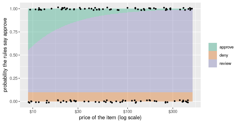
Every dot is a request. With a reader this sure of itself, almost every dot sits on the top or bottom edge, where the map says "approve" or "deny" at any price. The middle band, where a person reads it, is for split votes, and the dearer the item, the wider the band.

What votes can't see¶

Which decisions were still wrong, and how sure was the model about them?

votes |>
  mutate(decision_made = policy(.pred_class, days_since_delivery, final_sale)) |>
  filter(decision_made != decision) |>
  select(item, price, p, state, .pred_class, decision)

# A tibble: 1 × 6
  item       price     p state .pred_class   decision
  <chr>      <dbl> <dbl> <fct> <fct>         <fct>   
1 wool throw  13.3     1 used  opened_unused deny

Look at p for any row there. If it's in between, the rule saw the doubt and judged the item too cheap for a review to be worth $4: a risk taken on purpose, and priced. If it's 0 or 1, all five votes agreed, and were wrong. Votes measure how consistent a model is, not whether it's right, and a model that misreads a message the same way five times looks certain. The expected-cost rule can't catch what looks certain. That's called being badly calibrated, and the only way to know how badly is to check, on labelled rows, how often "five out of five" is really right:

votes |>
  group_by(p) |>
  summarise(requests = n(), rules_said_approve = mean(decision == "approve"))

# A tibble: 2 × 3
      p requests rules_said_approve
  <dbl>    <int>              <dbl>
1     0       57              0    
2     1       63              0.984

If "unanimous approve" is right only 98% of the time, you can tell the rule so: treat 1 as 0.98 and 0 as 0.02. Then any confident approval of an item dear enough (0.02 × price > $4, so above $200) goes to a person:

outcome(choose(pmin(pmax(votes$p, 0.02), 0.98), votes$price), "expected cost, votes capped at 2%-98%")

# A tibble: 1 × 5
  strategy                         reviews wrong_approvals wrong_denials dollars
  <chr>                              <int>           <int>         <int>   <dbl>
1 expected cost, votes capped at …      15               1             0    73.3

Is that worth it? The table says. Capping buys insurance against a confident mistake on an expensive item, and pays for it in reviews of expensive items the model got right. Whether it pays off depends on how often the confident mistakes happen and how dear they are, which is exactly what your costs and your labelled rows are for.

A model built for decisions: Jev¶

Everything so far used language models, which are built to write text, and squeezed a probability out of them by asking five times. TypeSafe's Jev is built the other way round. It writes no text at all. It answers typed questions (pick one of these options, yes or no, a score on a scale) with a probability for every possible answer, and it is trained so those probabilities are calibrated: of all the answers it gives at 80%, about 80% should be right. That is exactly what choose() needs.

It also costs almost nothing ($0.042 per million tokens read, and nothing for its answers) and answers in a fraction of a second. In functai it's just another model, because item_state is already a typed question with a set of answers:

jev_state <- update(item_state, lm = "jev-latest")

read_jev <- augment(jev_state, refunds)
read_jev |> select(state, .pred_class, .pred_unopened:.pred_faulty)

# A tibble: 120 × 8
   state .pred_class .pred_unopened .pred_opened_unused .pred_used .pred_damaged
   <fct> <fct>                <dbl>               <dbl>      <dbl>         <dbl>
 1 wron… wrong_item            0                   0             0             0
 2 wron… wrong_item            0                   0             0             0
 3 faul… faulty                0                   0             0             0
 4 faul… faulty                0                   0             0             0
 5 used  used                  0                   0             1             0
 6 faul… faulty                0                   0             0             0
 7 open… opened_unu…           0.02                0.98          0             0
 8 wron… wrong_item            0                   0             0             0
 9 faul… faulty                0                   0             0             0
10 unop… unopened              0.99                0.01          0             0
# ℹ 110 more rows
# ℹ 2 more variables: .pred_wrong_item <dbl>, .pred_faulty <dbl>

One call a row, and the probabilities come with the answer: no votes. How often is its reading right, next to gpt-6-luna's majority of five?

tibble(model = c("gpt-6-luna, 5 votes", "jev-latest, 1 call"),
       state_read_right = c(mean(votes$.pred_class == refunds$state), mean(read_jev$.pred_class == refunds$state)))

# A tibble: 2 × 2
  model               state_read_right
  <chr>                          <dbl>
1 gpt-6-luna, 5 votes            0.983
2 jev-latest, 1 call             0.983

The real test is the calibration check that votes failed: group the answers by how sure Jev said it was, and see how often each group was right.

read_jev |>
  mutate(sure = pmax(.pred_unopened, .pred_opened_unused, .pred_used, .pred_damaged, .pred_wrong_item, .pred_faulty),
         said = cut(sure, c(0, 0.8, 0.95, 0.99, 1), include.lowest = TRUE)) |>
  group_by(said) |>
  summarise(answers = n(), right = mean(.pred_class == state))

# A tibble: 4 × 3
  said        answers right
  <fct>         <int> <dbl>
1 [0,0.8]           6 0.833
2 (0.8,0.95]        8 0.875
3 (0.95,0.99]      24 1    
4 (0.99,1]         82 1

The answers it was very sure of were right, and its mistakes, if any, sit among the answers it was less sure of: its doubt is where the errors are, which is what votes could not promise. With 120 rows the lower groups hold a handful of answers each, so read this as a sanity check, not a measurement; checking calibration properly takes a few hundred labelled rows. And its probabilities spread over the whole range, instead of piling up at 0 and 1. The same functions from above turn them into decisions, because the columns have the same names:

read_jev <- read_jev |> mutate(p = p_approve(read_jev), action = choose(p, price))
outcome(read_jev$action, "expected cost, jev-latest")
read_jev |> filter(action == "review") |> select(item, price, p, state, .pred_class)

# A tibble: 1 × 5
  strategy                  reviews wrong_approvals wrong_denials dollars
  <chr>                       <int>           <int>         <int>   <dbl>
1 expected cost, jev-latest       3               0             0      12
# A tibble: 3 × 5
  item            price     p state      .pred_class
  <chr>           <dbl> <dbl> <fct>      <fct>      
1 wool throw       13.3  0.23 used       used       
2 coffee grinder  251.   0.17 used       used       
3 ceramic planter 190.   0.9  wrong_item wrong_item

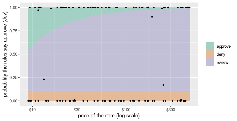
On the map, most of Jev's requests still sit at the edges: it was sure, and right. But a few now sit in between, the ones it was honestly unsure about, and there the map can act, sending the dear ones to a person:

#| fig-height: 3.6
ggplot(map, aes(price, p)) +
  geom_raster(aes(fill = action), alpha = 0.35) +
  geom_point(data = read_jev, aes(price, p), size = 1) +
  scale_fill_manual(values = c(approve = "#1b9e77", deny = "#d95f02", review = "#7570b3")) +
  scale_x_log10(labels = scales::label_dollar(accuracy = 1)) +
  labs(x = "price of the item (log scale)", y = "probability the rules say approve (Jev)", fill = NULL)

TypeSafe's advice for Jev is the design of this whole tutorial: ask it narrow questions a knowledgeable person could answer in a few seconds (what state is this item in?), and combine the answers with logic in your code (policy(), choose()). Jev can't write a reply to the customer or explain itself in prose; for that you'd still call a language model. For the decision itself, a model that measures its doubt is the right tool.

When the reader is weaker¶

Here's the same pipeline with gpt-5.4-nano, the small model of six months ago, which tutorial 5 found a clearly worse reader:

votes_nano <- augment(update(item_state, lm = "gpt-5.4-nano"), refunds, samples = 5)
votes_nano <- votes_nano |> mutate(p = p_approve(votes_nano), action = choose(p, price))

votes_nano |> summarise(state_read_right = mean(.pred_class == state))

bind_rows(
  outcome(with(votes_nano, policy(.pred_class, days_since_delivery, final_sale)), "trust nano's majority"),
  outcome(votes_nano$action, "expected cost, gpt-5.4-nano")
)

# A tibble: 1 × 1
  state_read_right
             <dbl>
1            0.917
# A tibble: 2 × 5
  strategy                    reviews wrong_approvals wrong_denials dollars
  <chr>                         <int>           <int>         <int>   <dbl>
1 trust nano's majority             0               0             0       0
2 expected cost, gpt-5.4-nano       3               0             0      12

A worse reader made far fewer wrong decisions than wrong readings. Many misreadings don't change the decision: "used" and "opened but unused" are both a "no" after 30 days, "damaged" and "faulty" both a "yes" within 60. What you should measure is the decision, because that's what costs money. Measuring only the reading would have made this model look much worse than it is at the job.

All the strategies, in dollars¶

all_strategies <- bind_rows(
  baselines,
  outcome(direct, "the model decides"),
  outcome(two_step, "the model reads, R decides"),
  outcome(votes$action, "expected cost, gpt-6-luna"),
  outcome(choose(pmin(pmax(votes$p, 0.02), 0.98), votes$price), "expected cost, capped, gpt-6-luna"),
  outcome(read_jev$action, "expected cost, jev-latest"),
  outcome(votes_nano$action, "expected cost, gpt-5.4-nano")
)
all_strategies |> arrange(dollars)

# A tibble: 9 × 5
  strategy                         reviews wrong_approvals wrong_denials dollars
  <chr>                              <int>           <int>         <int>   <dbl>
1 expected cost, jev-latest              3               0             0    12  
2 expected cost, gpt-5.4-nano            3               0             0    12  
3 the model decides                      0               1             0    13.3
4 the model reads, R decides             0               1             0    13.3
5 expected cost, gpt-6-luna              0               1             0    13.3
6 expected cost, capped, gpt-6-lu…      15               1             0    73.3
7 a person reads everything            120               0             0   480  
8 deny everything                        0               0            62  2480  
9 approve everything                     0              58             0  7114.

Remember what isn't in those dollars: the model calls themselves. They are in the log, and they are small:

prices <- tribble(
  ~model,         ~input, ~output,   # dollars per million tokens, 2026-09-27
  "gpt-6-luna",     0.10,    0.50,
  "gpt-5.4-nano",   0.20,    1.25,
  "jev-latest",    0.042,    0       # Jev charges only for what it reads
)

calls(folder = log_folder) |>
  left_join(prices, by = "model") |>
  group_by(model) |>
  summarise(calls = n(), dollars = sum(input_tokens * input + (total_tokens - input_tokens) * output, na.rm = TRUE) / 1e6)

# A tibble: 3 × 3
  model        calls dollars
  <chr>        <int>   <dbl>
1 gpt-5.4-nano   600 0.0333 
2 gpt-6-luna     720 0.0299 
3 jev-latest     120 0.00238

If nobody wrote the rules down¶

Sometimes there's no written policy, only past decisions: staff decided case by case, and you want to know what rule they were following. That's a job for a classic decision model: a decision tree, which learns yes/no questions from past cases. The model reads the state; the tree learns the rules from the history:

library(parsnip)
library(rsample)

read <- votes |> mutate(state_read = .pred_class)

set.seed(2026)
halves <- initial_split(read, prop = 1/2, strata = decision)
history <- training(halves)     # past decisions to learn from
incoming <- testing(halves)     # new requests to decide

tree <- decision_tree(mode = "classification", tree_depth = 4, min_n = 5) |>
  set_engine("rpart") |>
  fit(decision ~ state_read + days_since_delivery + final_sale + price, data = history)

#| fig-height: 4.5
wrap <- function(x, labs, digits, varlen, faclen)     # long lists of states, over several lines
  sapply(strwrap(gsub(",", ", ", labs), 26, simplify = FALSE), paste, collapse = "\n")

rpart.plot::rpart.plot(extract_fit_engine(tree), roundint = FALSE, type = 4, extra = 2, branch = 0.4,
                       fallen.leaves = TRUE, box.palette = "GnRd", split.fun = wrap)

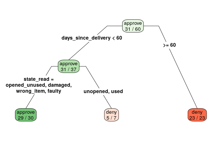
Read the picture from the top: each branch is labelled with the answer that leads down it; each box shows the decision there, and how many of the past requests that reached it had that decision, out of how many.

The same tree as rules, one line per leaf, is easier to put next to a policy. The number is the share of past requests there that were denied:

rpart.plot::rpart.rules(extract_fit_engine(tree), roundint = FALSE)

 decision                                                                                                
     0.03 when days_since_delivery <  60 & state_read is opened_unused or damaged or wrong_item or faulty
     0.71 when days_since_delivery <  60 & state_read is                                 unopened or used
     1.00 when days_since_delivery >= 60

Put its questions next to the rules in ?refunds. Which lines did it find? Which did it miss, or invent from the accidents of sixty past cases? And how well does it decide the other sixty, next to the written rules?

incoming |>
  mutate(tree = predict(tree, incoming)$.pred_class,
         written_rules = policy(state_read, days_since_delivery, final_sale)) |>
  summarise(tree = mean(tree == decision), written_rules = mean(written_rules == decision))

# A tibble: 1 × 2
   tree written_rules
  <dbl>         <dbl>
1 0.817             1

Sixty cases are not enough to learn four rules with three different time limits. The tree is still useful: it's a readable summary of what people actually did, and where it disagrees with what you think the policy is, you've found something to talk about. But when the rules can be written, write them.

Your turn¶

Change lost_customer to $10 and then $200. How does the map change? Which strategy wins at each value?
Add a fourth action: ask gpt-6-sol to read the state again, at a cost of about $0.001, and send to a person only when the two readers disagree. How much does it save over reviewing every unsure request?
Ask Jev atomic yes/no questions instead of one choice: a function with opened + used + broken_on_arrival ~ message, each described(logical(), "Has the customer opened the package?") and so on, one question each. Write the policy on those answers. Is it as accurate? Is it easier to explain?
Fit the tree on all 120 rows. Does it find the final-sale rule? Why is that rule hard to learn from this data? (count(refunds, final_sale, decision) is a hint.)

What you learned¶

A decision model is a choice with costs. Write the costs down; they matter more than the last point of accuracy.
Let the model read and R rule: policy() is exact, testable, explainable, and changes without touching the prompt.
samples = 5 gives votes; push their shares through the policy to get the probability of each decision.
Choose the action with the lowest expected cost. The same doubt means "approve" for a mug and "ask a person" for an espresso machine.
Votes are rough probabilities, and a consistently wrong model looks certain: check on labelled rows how often "unanimous" is right, and cap the probabilities accordingly.
A model built for decisions, like TypeSafe's Jev (lm = "jev-latest"), answers a typed question with a calibrated probability for every answer, in one call; augment() gives them as .pred_ columns, ready for the expected-cost rule.
Measure decisions, not readings: many misreadings don't change the decision.
A decision tree learns rules from past decisions; it needs far more cases than writing the rules down.

Answers to the check at the top. (1) Because its 3% of mistakes may be the expensive ones (a wrong approval on a $450 machine costs more than a hundred reviews of mugs); judge it in dollars. (2) With p = 0.8: for the $400 machine, approving risks 0.2 × $400 = $80, more than a $4 review, so a person looks; for the $12 mug, approving risks $2.40, less than a review, so approve. (3) Exact arithmetic on the facts, a reason for every decision, a policy you can test and change without the model, and a probability you can reason with. (4) Five identical answers only say the model is consistent; it can be consistently wrong. A model trained to be calibrated, like Jev, gives a probability per answer that you can check against labelled rows, and use.

Next: 7. AI functions in tidymodels puts a language model in the same workflows, resampling and tuning as any other model.