You know how tidymodels works. You write a model specification,
fit() it on training data, predict() new data,
and score the predictions with yardstick. Swap one model for another and
nothing else in your code moves.
This vignette shows that a language model can be one of those models. You describe the task in a sentence, and it goes through the same four verbs, into the same workflows, through the same resampling and tuning. Along the way we’ll find out when it is worth it and what it costs, with real numbers from a real model.
library(tidymodels)
library(textrecipes)
library(functai)

log_folder <- tempfile("functai-calls-")
ai_config(lm = "gpt-4.1-mini", temperature = 0, log_calls = log_folder)
ai_config() chooses the model every AI function uses,
unless it says otherwise. temperature = 0 asks for its most
likely answer every time. log_calls writes each call down,
so we can count them at the end. To run this yourself, set
OPENAI_API_KEY (or name another model:
"claude-haiku-4-5", "gemini:gemini-2.5-flash",
a local "ollama:qwen3.5:0.8b").
The vocabulary, side by side
| tidymodels | with a language model |
|---|---|
multinom_reg() |
ai_model("classification", "the task, in a sentence") |
set_engine("glmnet") |
set_engine("functai", lm = "claude-haiku-4-5"): the
language model is the engine |
fit() estimates weights |
fit() reads the outcome’s levels and, if you ask, picks
worked examples. No weights, no calls. |
predict() computes |
predict() asks the model, one call per row, 8 at a
time |
penalty = tune() |
examples = tune(): how many training rows it sees as
worked examples |
type = "prob" |
type = "prob" when you ask for several answers per row
(samples) |
| free to predict | every prediction is a paid call |
The last line is the one to keep in mind. It shapes every choice below.
The data
tickets ships with functai: 80 messages to a small
homeware shop, each sent to one of four teams. The shop has house rules.
A parcel damaged on the way is shipping, not product.
A refund is billing. Those rules are exactly what a model
cannot guess.
tickets <- functai::tickets |> mutate(category = factor(category))
count(tickets, category)
#> # A tibble: 4 × 2
#>   category     n
#>   <fct>    <int>
#> 1 account     18
#> 2 billing     22
#> 3 product     18
#> 4 shipping    22

set.seed(2026)
split <- initial_split(tickets, prop = 0.5, strata = category)
train <- training(split)
test  <- testing(split)
Forty messages to learn from and forty to test on. That’s small, and on purpose: small labelled data is where most text problems start.
A classical baseline
First, the model you’d normally reach for. The recipe turns each message into word weights (tf-idf), and a penalised multinomial regression learns which words point to which team.
tfidf <- recipe(category ~ message, data = train) |>
  step_tokenize(message) |>
  step_tokenfilter(message, max_tokens = 300) |>
  step_tfidf(message)

glmnet_fit <- workflow() |>
  add_recipe(tfidf) |>
  add_model(multinom_reg(penalty = 0.01) |> set_engine("glmnet")) |>
  fit(train)

augment(glmnet_fit, test) |> accuracy(category, .pred_class)
#> # A tibble: 1 × 3
#>   .metric  .estimator .estimate
#>   <chr>    <chr>          <dbl>
#> 1 accuracy multiclass     0.625
62% right. That’s not bad for forty examples, but a model that learns words from forty messages has seen very few words.
The same four verbs, with a language model
ai_spec <- ai_model("classification", "Which team should answer this customer message?") |>
  set_engine("functai")
ai_spec
#> AI Model Specification (classification)
#>
#> Main Arguments:
#>   description = Which team should answer this customer message?
#>
#> Computational engine: functai
The description is the whole model: what you would tell a new colleague on their first day. Now fit it, and time it:
system.time(ai_fit <- fit(ai_spec, category ~ message, data = train))
#>    user  system elapsed
#>   0.006   0.000   0.007
ai_fit
#> parsnip model object
#>
#> <ai function> category ~ message
#>   Which team should answer this customer message?
#>   message   text
#>   category  one of account, billing, product, shipping
#>   model: gpt-4.1-mini
That took no time because nothing was called. Fitting read the
formula (the input is message), and it read the outcome’s
four levels (the only answers the model may give). The answers in
train were not used at all: this model starts “zero-shot”.
Predicting is where the work happens:
ai_pred <- augment(ai_fit, test)
#> Warning: probabilities are NA: one answer per row measures no probability
#> ℹ for them, answer each row several times: `set_engine("functai", samples = 5)` (costs 5
#>   calls a row)
ai_pred |> select(message, category, .pred_class)
#> # A tibble: 40 × 3
#>    message                                                            category .pred_class
#>    <chr>                                                              <fct>    <fct>
#>  1 Hi, my order A-1042 still hasn't arrived and it's been three week… shipping shipping
#>  2 I was charged twice for order B-2210, please fix this.             billing  billing
#>  3 The kettle lid doesn't close properly anymore after a month of us… product  product
#>  4 Tracking for C-3319 hasn't moved since Monday.                     shipping shipping
#>  5 I forgot my password and the reset email never comes.              account  account
#>  6 Box was crushed and the lamp inside is cracked. Order D-4001.      shipping shipping
#>  7 My coupon code SPRING10 didn't apply at checkout.                  billing  billing
#>  8 Can the cast iron pan go in the dishwasher?                        product  product
#>  9 Please delete my account and all my data.                          account  account
#> 10 Refund the blender please, it stopped working after two days.      billing  billing
#> # ℹ 30 more rows
ai_pred |> accuracy(category, .pred_class)
#> # A tibble: 1 × 3
#>   .metric  .estimator .estimate
#>   <chr>    <chr>          <dbl>
#> 1 accuracy multiclass     0.925
ai_pred |> conf_mat(category, .pred_class)
#>           Truth
#> Prediction account billing product shipping
#>   account        7       0       0        0
#>   billing        0      11       0        0
#>   product        2       0       9        1
#>   shipping       0       0       0       10
92% right, with no training at all. And augment() warned
that the probability columns are NA. That’s deliberate, and
the section on probabilities below explains it.
Which messages did it get wrong?
ai_pred |>
  filter(category != .pred_class) |>
  select(message, category, .pred_class)
#> # A tibble: 3 × 3
#>   message                                                  category .pred_class
#>   <chr>                                                    <fct>    <fct>
#> 1 Package arrived but the bowl inside was in three pieces. shipping product
#> 2 I can't find where to log out on the app.                account  product
#> 3 I get 'invalid token' every time I try to sign in.       account  product
Read them against the shop’s house rules. Anything that arrived broken is shipping, because the carrier pays. Every request for money back is billing. Problems that appear while using a product are product. Signing in and personal data are account. A model reading a message cold can’t know where this shop draws those lines, so it makes the reasonable call rather than the house call.
What did fit() make? A function
Under the parsnip wrapper, the fitted engine is an ordinary R function:
team <- extract_fit_engine(ai_fit)
team
#> <ai function> category ~ message
#>   Which team should answer this customer message?
#>   message   text
#>   category  one of account, billing, product, shipping
#>   model: gpt-4.1-mini
team("My card was charged twice for order B-2210.")
#> [1] billing
#> Levels: account billing product shipping
It is the function
ai(category ~ message, "Which team should answer this customer message?", .data = train)
writes: the formula you give fit() is the one you give
ai(). It is vectorised, so it also works outside
tidymodels, as a column in any dplyr verb:
test |>
  slice(1:4) |>
  mutate(team = team(message)) |>
  select(message, team)
#> # A tibble: 4 × 2
#>   message                                                             team
#>   <chr>                                                               <fct>
#> 1 Hi, my order A-1042 still hasn't arrived and it's been three weeks. shipping
#> 2 I was charged twice for order B-2210, please fix this.              billing
#> 3 The kettle lid doesn't close properly anymore after a month of use. product
#> 4 Tracking for C-3319 hasn't moved since Monday.                      shipping
Here the two worlds meet. The same object is a tidymodels model, fitted and tuned with the grammar you know, and a function you can call wherever you have text.
Comparing fairly
On forty test messages, a difference of a few points could be luck.
evaluate() scores any model, whether a workflow, a parsnip
fit or an AI function, and gives each score a 95% interval:
scores <- bind_rows(
  tidy(evaluate(glmnet_fit, test)) |> mutate(model = "glmnet on tf-idf (trained on 40)"),
  tidy(evaluate(ai_fit, test))     |> mutate(model = "gpt-4.1-mini (no training)")
)
scores |> select(model, estimate, conf.low, conf.high)
#> # A tibble: 2 × 4
#>   model                            estimate conf.low conf.high
#>   <chr>                               <dbl>    <dbl>     <dbl>
#> 1 glmnet on tf-idf (trained on 40)    0.625    0.470     0.758
#> 2 gpt-4.1-mini (no training)          0.9      0.769     0.960
ggplot(scores, aes(estimate, model)) +
  geom_pointrange(aes(xmin = conf.low, xmax = conf.high)) +
  scale_x_continuous(labels = scales::percent, limits = c(0, 1)) +
  labs(x = "right, with a 95% interval", y = NULL)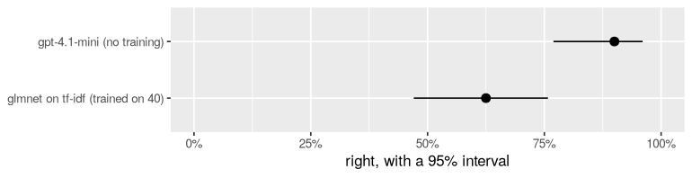
How often each model is right on the 40 test messages, with 95% intervals.
The intervals don’t overlap. With forty test messages that’s a big gap, and it means the difference is real, not luck.
In a workflow, resampled and tuned
A language model can learn from a few worked examples: a message and
its right team, shown before each question. examples is the
model’s tuning parameter. Here it is in a workflow, tuned by
cross-validation like any other:
ai_wf <- workflow() |>
  add_formula(category ~ message) |>
  add_model(
    ai_model("classification", "Which team should answer this customer message?",
             examples = tune()) |>
      set_engine("functai")
  )

set.seed(1)
folds <- vfold_cv(train, v = 5, strata = category)

tuned <- tune_grid(ai_wf, folds,
                   grid = tibble(examples = c(0, 2, 4, 8)),
                   metrics = metric_set(accuracy))
collect_metrics(tuned) |> select(examples, mean, std_err)
#> # A tibble: 4 × 3
#>   examples  mean std_err
#>      <dbl> <dbl>   <dbl>
#> 1        0 0.88   0.0561
#> 2        2 0.782  0.0317
#> 3        4 0.847  0.0476
#> 4        8 0.95   0.0306
Two things to notice.
The formula, not a recipe. A language model reads
the message itself. A recipe that turns it into word weights would take
the words away. So the workflow uses add_formula().
The metric set. tune’s default metrics include
roc_auc, which needs probabilities. One answer per row has
none (see below), so we ask for accuracy only.
Each value was fitted five times and predicted on eight held-out rows each time, so every mean above rests on forty answers. Read it against the standard errors, a few points each.
8 examples scored best, 7 points above none. Measured against the uncertainty of both scores, that gap is about 1.1 times its standard error: forty answers can’t tell it apart from luck. And 2 and 4 examples scored lower than none. A few examples can mislead as well as teach, because the model copies the pattern of whichever messages it happened to see.
The model already knows the language, so worked examples are only worth their price when they teach it something it can’t guess. Here that’s the shop’s house rules, and a handful of random rows rarely covers them.
last_fit() gives the honest final number: the chosen
setting, fitted on all of train, scored once on
test.
best <- select_best(tuned, metric = "accuracy")
best
#> # A tibble: 1 × 2
#>   examples .config
#>      <dbl> <chr>
#> 1        8 pre0_mod4_post0
final <- finalize_workflow(ai_wf, best) |>
  last_fit(split, metrics = metric_set(accuracy))
collect_metrics(final)
#> # A tibble: 1 × 4
#>   .metric  .estimator .estimate .config
#>   <chr>    <chr>          <dbl> <chr>
#> 1 accuracy multiclass       0.9 pre0_mod0_post0
90% on the test set with 8 examples, against 92% with none. The test set did not confirm the gain. That’s the winner’s curse: picking the best of four noisy scores favours whichever setting got lucky on these folds. Always check a tuned setting on data it never saw, as last_fit() does, before you pay for it: here, more examples per call bought nothing.
Probabilities, honestly
tidymodels models give type = "prob": a probability per
class, which roc_auc(), calibration plots and thresholds
need. OpenAI, Anthropic and Gemini don’t say how likely each answer is,
and functai never invents that number. That’s why augment()
above had NA probabilities.
What you can do is ask the same question several times. With
samples = 5, each message is answered five times at
temperature 1. The probability of a team is its share of those five
answers, and the class is the majority vote:
voter <- ai_model("classification", "Which team should answer this customer message?") |>
  set_engine("functai", samples = 5) |>
  fit(category ~ message, data = train)

votes <- augment(voter, test)
votes |> select(category, .pred_class, .pred_account:.pred_shipping) |> head()
#> # A tibble: 6 × 6
#>   category .pred_class .pred_account .pred_billing .pred_product .pred_shipping
#>   <fct>    <fct>               <dbl>         <dbl>         <dbl>          <dbl>
#> 1 shipping shipping                0             0             0              1
#> 2 billing  billing                 0             1             0              0
#> 3 product  product                 0             0             1              0
#> 4 shipping shipping                0             0             0              1
#> 5 account  account                 1             0             0              0
#> 6 shipping shipping                0             0             0              1
votes |> roc_auc(category, .pred_account:.pred_shipping)
#> # A tibble: 1 × 3
#>   .metric .estimator .estimate
#>   <chr>   <chr>          <dbl>
#> 1 roc_auc hand_till      0.981
Where did the five answers disagree?
votes |>
  filter(pmax(.pred_account, .pred_billing, .pred_product, .pred_shipping) < 1) |>
  select(message, category, .pred_class, .pred_account:.pred_shipping)
#> # A tibble: 3 × 7
#>   message    category .pred_class .pred_account .pred_billing .pred_product .pred_shipping
#>   <chr>      <fct>    <fct>               <dbl>         <dbl>         <dbl>          <dbl>
#> 1 My coupon… billing  billing               0             0.8           0.2            0
#> 2 Package a… shipping product               0             0             0.6            0.4
#> 3 I get 'in… account  product               0.2           0             0.8            0
Only 3 of 40 messages split the vote. 2 of the vote’s 3 mistakes are among them, so the split votes do point at messages a person should check.
This cost five calls per message; the class and the probabilities
share them. The probabilities come in steps of 0.2, and
gpt-4.1-mini is sure of itself most of the time. So
roc_auc here rewards the model for being right, more than
for knowing when it might not be. The fix for consistent mistakes isn’t
more votes. It’s teaching the rule: write it into the description, or
show it with worked examples that cover it.
The other way round: a classical model that learns from the language model
Swapping works in both directions. Say you had thousands of unlabelled messages. The language model can label them once, and a classical model can learn from those labels, then predict for free, forever, offline.
Here we pretend train has no labels: the language model
labels it, and glmnet learns from its answers instead of a person’s.
ai_labelled <- train |>
  select(message) |>
  mutate(category = team(message))

student <- workflow() |>
  add_recipe(recipe(category ~ message, data = ai_labelled) |>
               step_tokenize(message) |>
               step_tokenfilter(message, max_tokens = 300) |>
               step_tfidf(message)) |>
  add_model(multinom_reg(penalty = 0.01) |> set_engine("glmnet")) |>
  fit(ai_labelled)

bind_rows(
  tidy(evaluate(glmnet_fit, test)) |> mutate(labels = "a person's"),
  tidy(evaluate(student, test))    |> mutate(labels = "the language model's")
) |> select(labels, estimate, conf.low, conf.high)
#> # A tibble: 2 × 4
#>   labels               estimate conf.low conf.high
#>   <chr>                   <dbl>    <dbl>     <dbl>
#> 1 a person's              0.625    0.470     0.758
#> 2 the language model's    0.525    0.375     0.671
The language model’s labels matched a person’s on 95% of the training messages. The student learned from those and reached 52%, against 62% for the model trained on a person’s labels. The intervals overlap: with forty messages to learn from, both students are limited by how few messages they saw, far more than by who labelled them.
Forty messages is far too few for a word-counting model, whoever labels them. The pattern is what scales. Labelling 40,000 messages is 40,000 cheap calls, done once. The classical model trained on them then predicts for free, offline, in milliseconds. Before you trust it, measure the student against a few hundred rows a person labelled.
What this vignette cost
Every call was logged, so we can count them:
calls(folder = log_folder) |>
  summarise(calls = n(),
            input_tokens = sum(input_tokens),
            output_tokens = sum(output_tokens))
#> # A tibble: 1 × 3
#>   calls input_tokens output_tokens
#>   <int>        <dbl>         <dbl>
#> 1   525        64061          4725
A few cents with gpt-4.1-mini. Most calls came from
tuning (4 values × 40 rows) and from voting (5 × 40). Resampling and
tuning multiply calls like nothing else does, so choose small grids.
Rules of thumb
-
Start zero-shot. A description and
fit()cost nothing. Measure it before you tune it. -
Measure with intervals. Small test sets make small
differences meaningless;
evaluate()says how small. - Use the formula, not a word recipe, for an AI model in a workflow.
-
Ask for probabilities only when you need them
(
samples), and for tuning without them, usemetric_set(accuracy). -
Keep
temperature = 0for scoring. Answers can still vary a little from run to run; that’s part of why intervals matter. -
Call the engine directly when you just want
answers:
extract_fit_engine(fit)is a vectorised R function. - Let a language model label, and a classical model learn when you need to predict millions of rows.